
Sommaire de l’article
Un lot est libéré parce que le contrôle qualité final est conforme, alors même que personne ne peut dire à quel point ce lot ressemblait au comportement normal du procédé une heure plus tôt. Une investigation de déviation cite une cause plausible sans jamais démontrer laquelle des dizaines de variables corrélées a réellement bougé en premier. Une proposition de changement de procédé est débattue sans qu'aucune estimation bornée de son effet ne soit produite. Trois situations, un manque commun : le produit a un état, mais cet état n'est ni localisé, ni expliqué, ni projeté.
L'hypothèse de recherche H1 est la suivante : un état de contrôle pharmaceutique devient connaissable de manière défendable lorsque trois couches liées sont maintenues : une estimation phase-aware de l'état courant du produit/procédé par rapport à une trajectoire normale représentative ; une couche d'attribution identifiant quels attributs matière, paramètres procédé ou attributs qualité expliquent l'écart et quand il est apparu ; et une couche prédictive consciente de sa validité estimant comment des changements candidats pourraient déplacer l'état.
H1 est conditionnellement soutenue au niveau du mécanisme. La preuve démontre que des méthodes multivariées phase-aware peuvent localiser un lot par rapport à une trajectoire d'évolution normale, que des analyses de résidus/contribution peuvent identifier des moteurs statistiques et leur chronologie, et que des modèles PAT peuvent estimer des attributs produit proches du temps réel. De petites expériences de contrôle adaptatif montrent comment un état mesuré peut être relié à un actionneur. La preuve n'établit pas de métrique universelle d'état de contrôle valable sur tout le cycle de vie, ni une réduction regroupée du taux de lots rejetés, ni une garantie causale que le contributeur statistique le plus élevé est la cause physique racine.
Frontière avec la partie 2.5 : cette synthèse est un problème d'observabilité et d'état de décision — localiser l'état courant, expliquer l'écart et exposer un mouvement plausible sous changements candidats. La partie « état de contrôle opérationnel » est un problème de modèle d'exploitation — transformer ces observations en une cadence continûment exécutée de contrôles, d'escalade, de gouvernance, d'intervention et de vérification. La figure 8 ci-dessous touche cette frontière ; elle n'est utilisée ici que pour démontrer la sensibilité d'un actionneur, pas pour développer l'argument périodique-versus-opérationnel.
Partie 1 — Savoir où en est le produit
The Signal and the Noise de Nate Silver est utilisé ici uniquement comme dispositif de cadrage rhétorique : la table des matières visible par l'éditeur identifie « Desperately Seeking Signal » à partir de la page 142. Silver n'est pas une autorité de fabrication pharmaceutique ; les affirmations techniques de cette section proviennent de sources évaluées par les pairs.
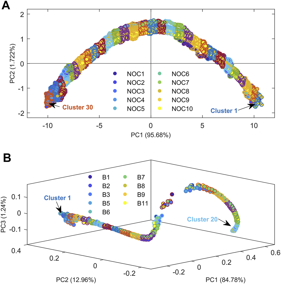 Rocha de Oliveira & de Juan, Frontiers in Analytical Science, 2022 — sous licence CC BY 4.0.
« PCA score plot for the online NIR observations showing the NOC batch process trajectories and local clusters found by k-means for (A) Process 1, fluidized bed drying, and (B) Process 2, gasoline blend distillation. The inner part of the circles is colored according to the related NOC batch, whereas the outer part reflects the observations included in every cluster and, hence, in the related local MSPC model. »
Le panneau A montre dix lots NOC de séchage en lit fluidisé partitionnés en 30 régions locales de progression ; le panneau B montre un second procédé en trois dimensions avec 20 clusters. Le graphique encode où se situe une observation le long d'une trajectoire d'évolution normale, plutôt que si un seul point final réussit.
Une fois la trajectoire de référence localement définie, chaque nouvelle observation en ligne peut être projetée sur ces modèles locaux et représentée comme une paire : progression de procédé estimée et distance Q réduite par rapport à la région de référence locale. La limite de contrôle normalisée est 1. L'idée clé n'est pas la seule détection d'anomalie : c'est la localisation d'état conditionnée par la phase. Un spectre de séchage en phase précoce ne devrait pas être comparé à un spectre de fin de procédé simplement parce que les deux appartiennent au même lot.
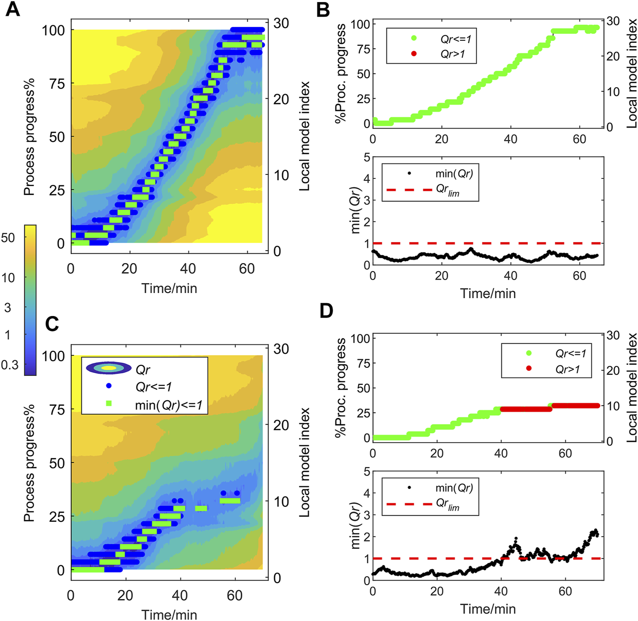 Rocha de Oliveira & de Juan, Frontiers in Analytical Science, 2022 — sous licence CC BY 4.0.
« Qr-based MSPC charts for fluidized bed drying (Process 1) batch NOC1 (A and B) and batch Fault1 (C and D). (A and C) Contour plots of the Qr values calculated after the projection of each NIR observation onto the local MSPC models. Blue dots show values of Qr < 1 (control limit), green squares the min (Qr < 1). (B and D) Charts show the min (Qr) value (bottom panel) and the related process progress associated with it (top panel) for every batch observation. In the process progress plot, NOC observations are displayed in green and faulty observations in red. »
NOC1 reste sous la limite de contrôle tout au long du lot ; Fault1 commence à produire des observations au-dessus de la limite à environ 40 minutes. L'état courant d'un lot peut ainsi être exprimé conjointement comme une progression et une distance multivariée par rapport à la région de fonctionnement normal locale.
Shi et al. (2021) passent en revue la modélisation multivariée à travers la fabrication de comprimés et couvrent explicitement la compréhension, le monitoring et le contrôle de procédé. Kim et al. (2021) passent en revue les outils PAT comme couche de stratégie de contrôle pour la vérification continue de procédé et l'information qualité en temps quasi réel. Les deux soutiennent la famille de méthodes ; aucun ne fournit une taille d'effet regroupée.
Une réponse défendable à « où en est le produit ? » exige donc un vecteur d'état combinant la phase de procédé, la distance multivariée à une région normale représentative, les estimations CQA/PAT pertinentes, et la validité du modèle et de la mesure. Un résultat de spécification finale seul est trop tardif et de dimension trop faible.
Partie 2 — Savoir pourquoi il en est là
La même liste de livres autorisés identifie « What You Don't Know Can Hurt You » à partir de la page 412. Le titre du chapitre est utilisé comme un accroche pour l'incertitude visible et les variables explicatives manquantes ; ce n'est pas une preuve pour l'analyse de cause racine pharmaceutique.
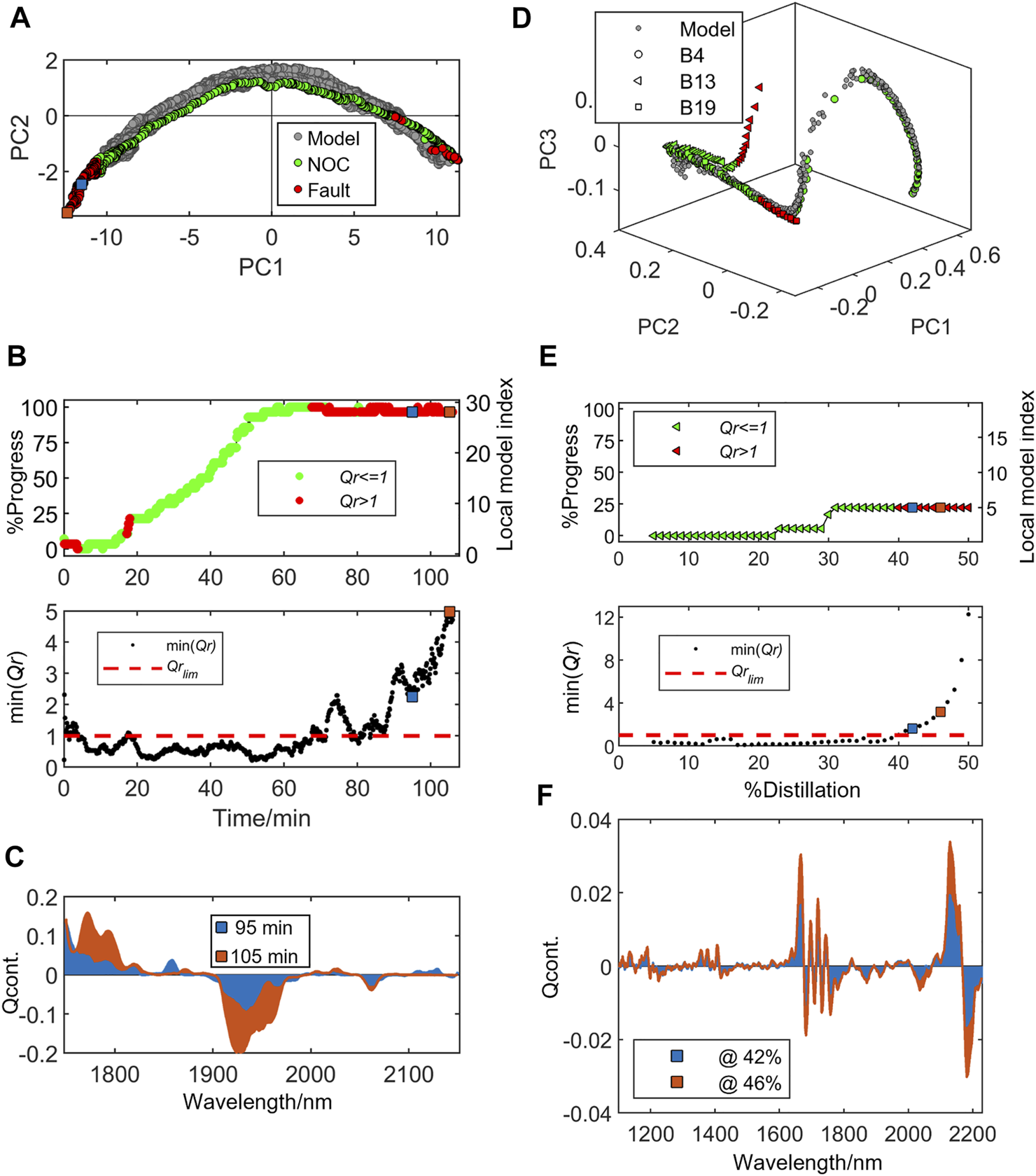 Rocha de Oliveira & de Juan, Frontiers in Analytical Science, 2022 — sous licence CC BY 4.0.
« Online tracking of new batch evolution using the local MSPC models for process 1 (fluidized bed drying) left plots (A to C) and process 2 (gasoline blend distillation) right plots (D to F). (A) Process 1 PCA score plot showing the training NOC batches trajectories (gray dots) and validation batch Fault2 trajectory in green (NOC observations) and red dots (faulty observations). (B) MSPC chart showing the process progress (top panel) and min (Qr)-based MSPC chart. (C) Q contribution (Qcont.) plots for two faulty observations at 95 and 105 min of batch Fault2 drying time represented by the blue and orange squares in the MSPC control chart. (D) Process 2 PCA score plot showing the training NOC batches trajectories (gray dots) and three validation batches (B4 circles, B13 triangles and B19 squares) trajectories in green (NOC observations) and red dots (faulty observations). (E) MSPC chart showing faulty batch B13 process progress (top panel) and min (Qr)-based MSPC chart. (F) Q contribution (Qcont.) plots for two faulty observations at 42 and 46% of distillation represented by the blue and orange squares in the MSPC control chart. »
Pour le lot de séchage défectueux, la trajectoire d'état passe de normale à anormale et des graphiques de contribution sont montrés à 95 et 105 minutes ; un exemple parallèle de distillation présente des observations anormales à 42 % et 46 % de progression. La même couche de monitoring répond ainsi à où en est le procédé, s'il sort de la région de référence locale, et quelles variables mesurées pilotent l'écart — sans que ces contributions statistiques soient automatiquement des mécanismes causaux.
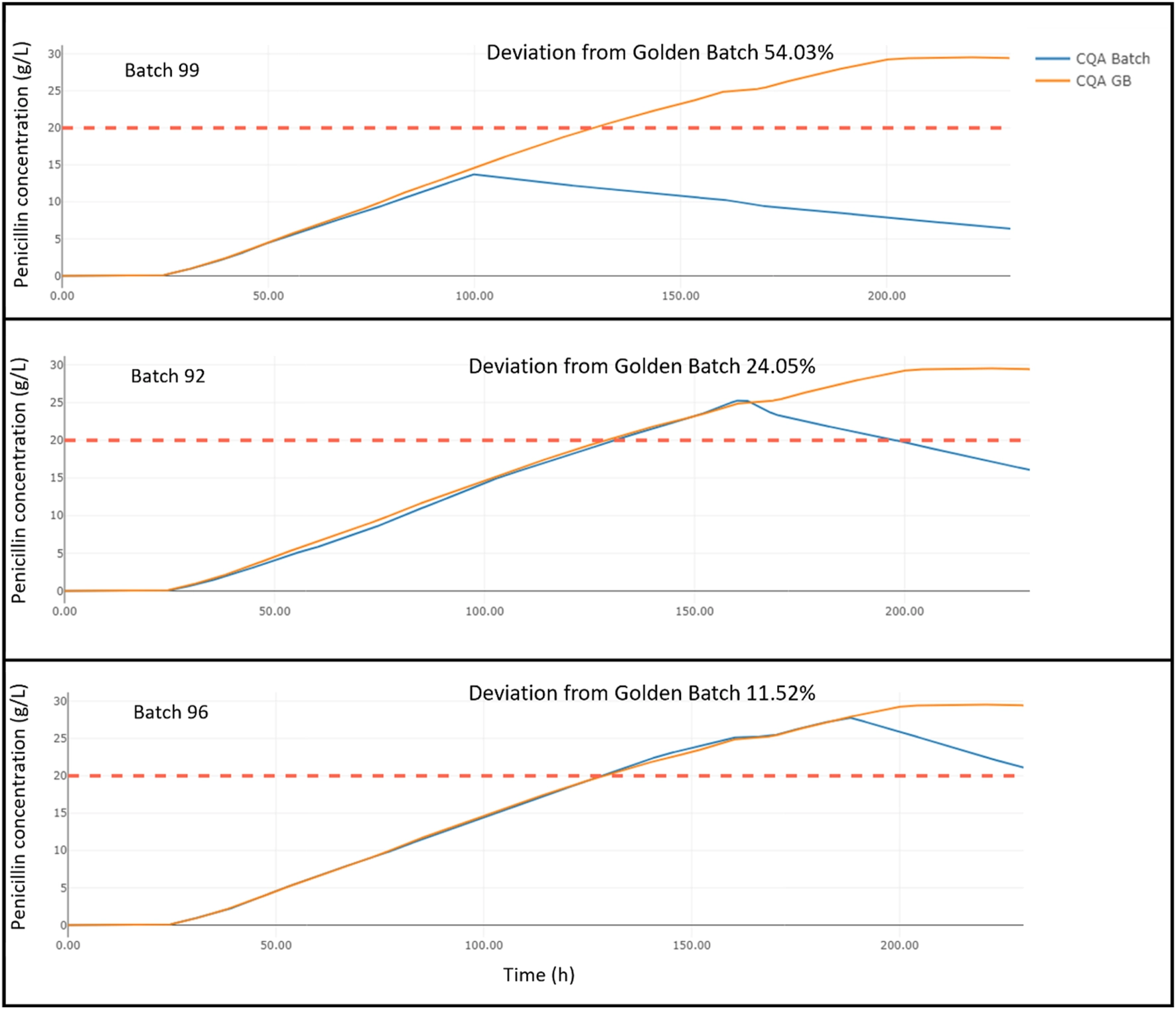 Luo et al., Frontiers in Manufacturing Technology, 2024 — sous licence CC BY 4.0.
« Comparison of penicillin production deviation across batches 99, 92, and 96 against golden batch standard. »
Sur un jeu simulé de 100 lots (67 sains, 33 malsains, échantillonnage toutes les 12 minutes), les déviations agrégées sélectionnées sont d'environ 54,03 %, 24,05 % et 11,52 % pour les lots 99, 92 et 96. Ces pourcentages sont spécifiques à la méthode et au jeu de données simulé ; ils ne sont pas des probabilités de risque transférables.
 Luo et al., Frontiers in Manufacturing Technology, 2024 — sous licence CC BY 4.0.
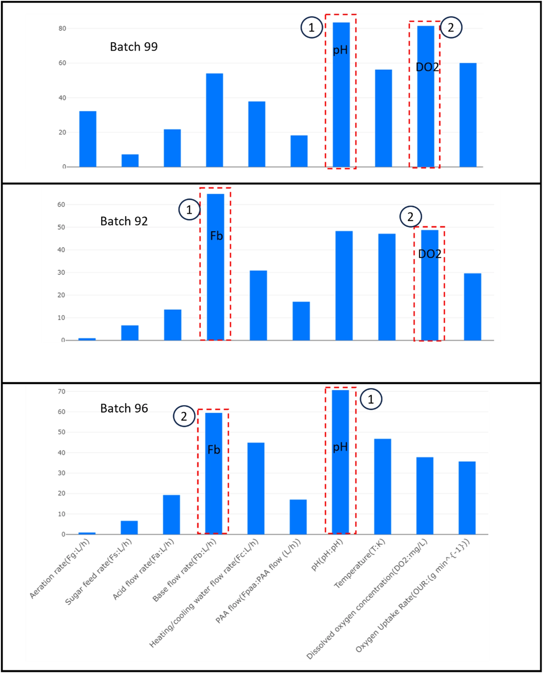
« Key contributors to deviation in penicillin production for batches 99, 92, and 96. »
Le classement de contribution diffère par lot : pH et oxygène dissous dominent pour le lot 99, débit de base et oxygène dissous pour le lot 92, pH et débit de base pour le lot 96. Un état anormal peut ainsi être décomposé en un profil de moteurs spécifique au lot plutôt que représenté par une alarme indifférenciée unique — mais une association classée ne prouve pas la causalité physique.
 Luo et al., Frontiers in Manufacturing Technology, 2024 — sous licence CC BY 4.0.
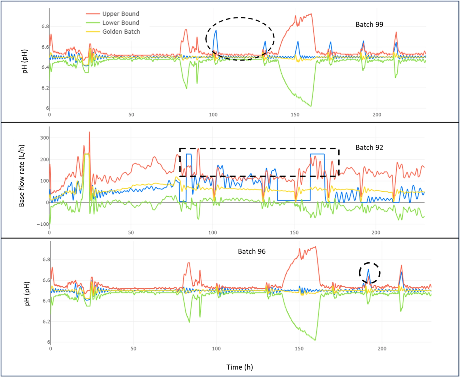
« Analysis of topmost significant contributor to deviations over time for penicillin production batches 99, 92, and 96. »
Le principal contributeur trace des départs de pH autour de 100 et 135 heures pour le lot 99, des départs répétés de débit de base entre environ 80 et 180 heures pour le lot 92, et un pic de pH autour de 190 heures pour le lot 96. Les traces temporelles aident à déterminer quand le système a commencé à bouger et si l'écart est transitoire, répété ou persistant — à condition de disposer de profils de référence représentatifs et d'une méthode d'alignement défendable.
Un graphique de contribution répond : quelle variable mesurée contribue le plus au résidu du modèle ? Il ne répond pas de lui-même : quel mécanisme physique a causé l'événement ? Des variables corrélées, des causes communes, un biais de capteur et une erreur d'alignement peuvent déplacer l'importance apparente. La chaîne correcte est donc : contributeur statistique → hypothèse causale bornée → preuve orthogonale → conclusion d'investigation responsable.
« Pourquoi » devient défendable lorsque la magnitude de déviation, la contribution par variable et le temps d'apparition sont reliés à une référence représentative puis testés par une preuve physique/procédé. Le modèle resserre l'investigation ; il ne doit pas la clore automatiquement.
Partie 3 — Savoir ce qui pourrait le faire bouger
La table des matières du livre autorisé identifie « Less and Less and Less Wrong » à partir de la page 232. Elle n'est utilisée ici que comme accroche pour la correction itérative de modèle et la réduction d'incertitude.
 Dietrich et al., Frontiers in Bioengineering and Biotechnology, 2025 — sous licence CC BY 4.0.
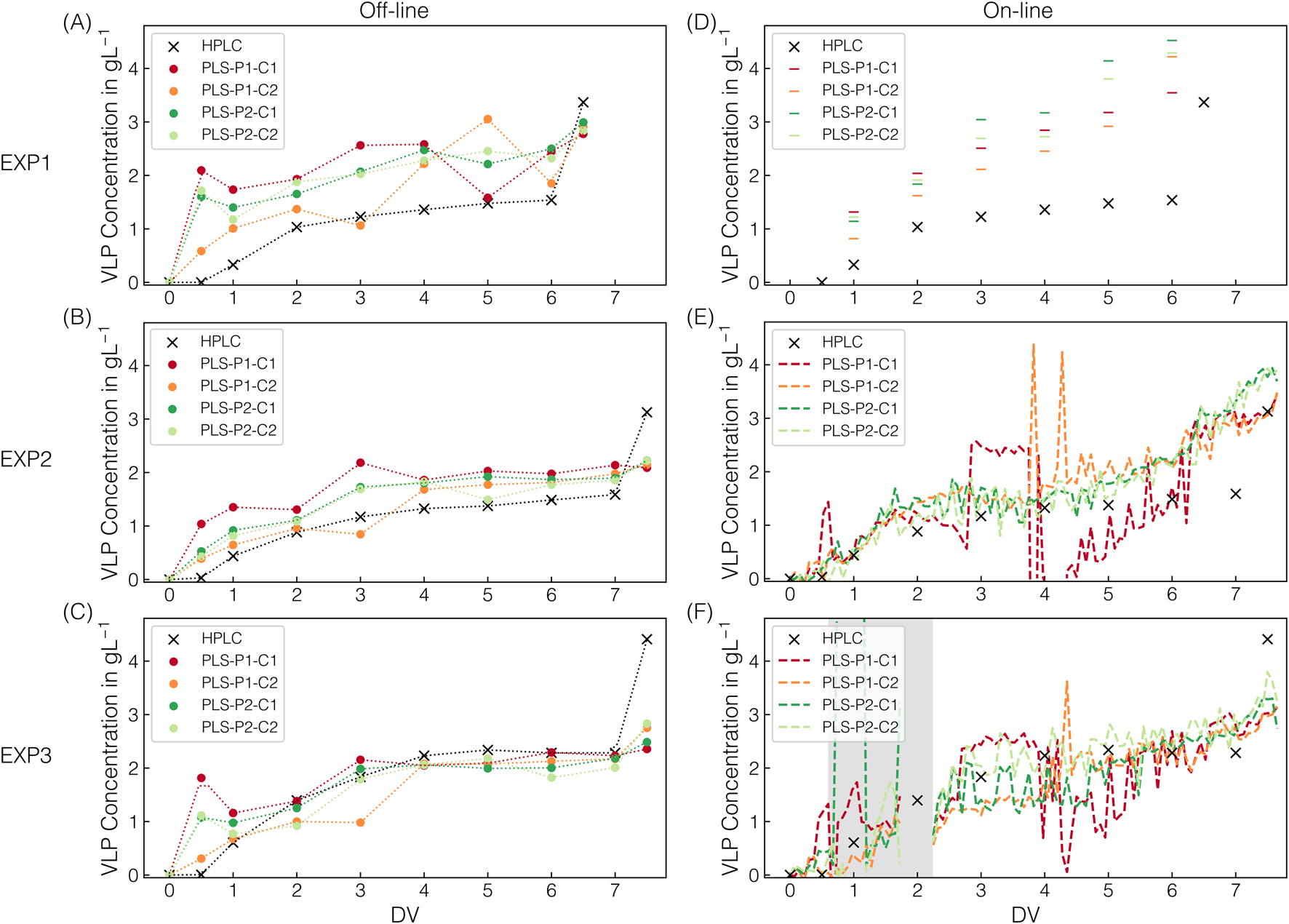
« VLP model predictions. Next to HPLC-derived VLP concentrations, the predicted VLP concentrations are shown for all CFF runs. The predictions derived from individual Raman measurements at 1,250 ms exposure time. Predictions from off-line and on-line measurements in semi-continuous (EXP1) or continuous (EXP2–3) acquisition mode are shown in (A–C) and (D–F), respectively, along with their corresponding color assignments for the models used. The models differ in pre-cropping and cropping operations, with their respective intervals P1/P2 and C1/C2. Dotted lines (off-line) serve solely as visual guides to facilitate interpretation. The dashed lines (on-line) represent continuous prediction. Predictions by defective spectra are highlighted with dark-gray shaded areas. »
Les zones grisées marquent les périodes de spectres défectueux, où le choix de prétraitement et de recadrage change la qualité de prédiction. Le PAT quasi temps réel peut donc estimer un attribut produit tout en exposant simultanément les périodes où la mesure ou le modèle n'est pas fiable ; une estimation sans indicateur de validité crée une fausse confiance.
Ce point est crucial : l'état de produit estimé doit porter un état de validité de mesure. Un transfert de modèle imparfait ou un spectre défectueux peut dégrader silencieusement une estimation qui, en apparence, continue de produire un nombre.
 Gasset et al., Frontiers in Bioengineering and Biotechnology, 2024 — sous licence CC BY 4.0.
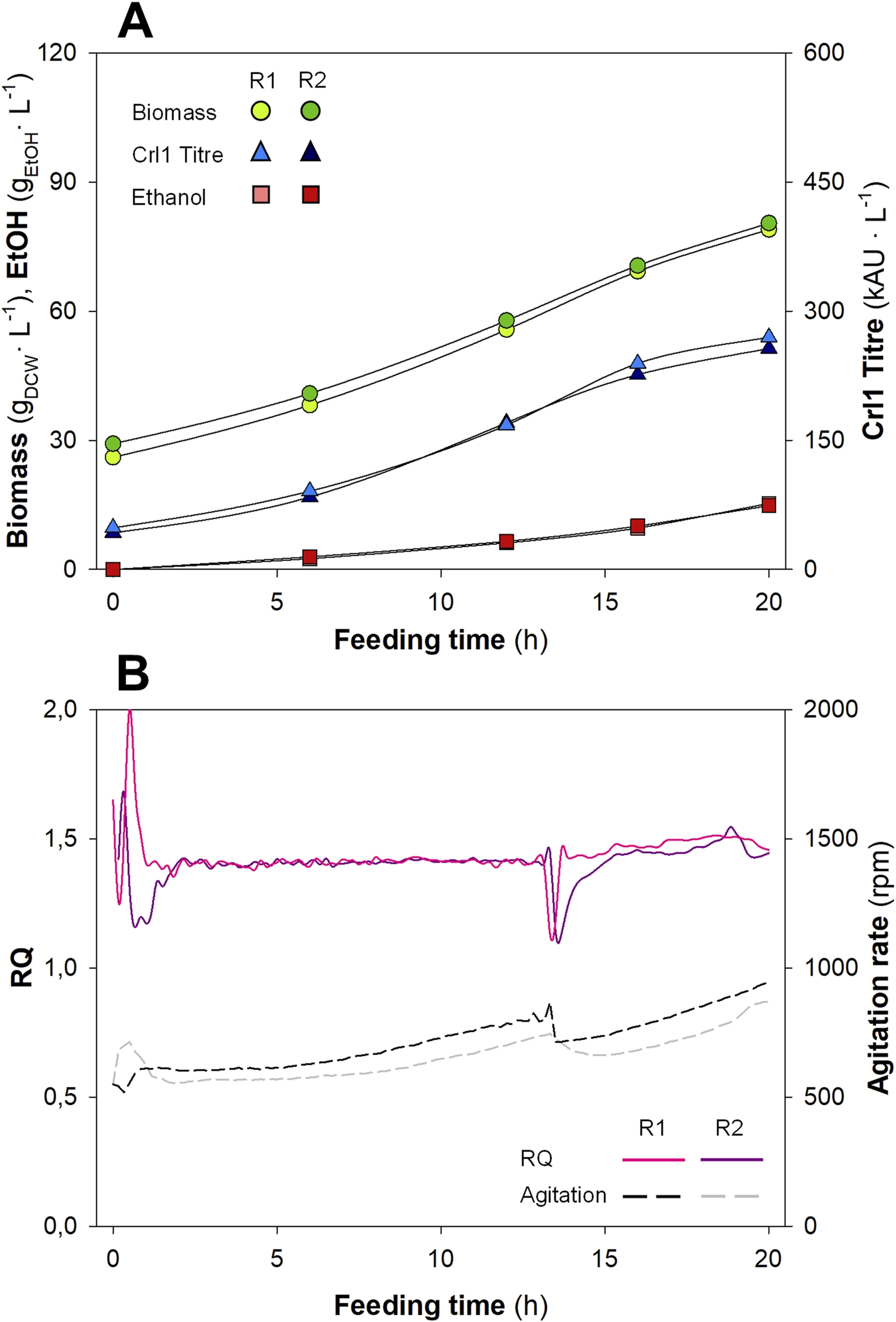
« Key process parameters (Biomass, Ethanol, and Crl1), agitation rate, and RQ for the biological replicates (R1 and R2) with the AI-aided Adaptive Proportional Control (AI-APC) strategy. (A) Biomass concentration, gDCW·L⁻¹; Crl1 Titre, kAU·L⁻¹; EtOH, Ethanol concentration, g·L⁻¹. (B) Off-line RQ calculation (continuous lines); agitation rate (discontinuous lines, rpm). »
Deux réplicats biologiques montrent une biomasse finale proche de 79 à 80 gDCW/L, un titre Crl1 autour de 257 à 270 kAU/L et un éthanol autour de 15 g/L, tandis que le RQ reste proche de sa cible. C'est la preuve la plus proche de « ce qui pourrait le faire bouger » : l'actionneur est explicite et la réponse est observée — mais deux réplicats n'établissent pas une performance industrielle générale, et l'action en boucle fermée relève en partie de la partie « état de contrôle opérationnel ».
Une affirmation de mouvement devrait être exprimée comme un contrefactuel avec limites d'applicabilité, pas comme une recommandation inconditionnelle : « sous cette version de modèle, dans cette région de fonctionnement et cet état de validité de mesure, changer l'actionneur X de Δ est prédit pour déplacer les variables d'état Y dans l'horizon H ». La revue humaine et un repli sûr restent requis.
Architecture intégrée de la preuve
La preuve soutient un objet d'état de contrôle à sept couches :
- Identité : produit, lot, opération unitaire, équipement, lot de matière et version de modèle.
- Progression : temps écoulé plus estimation de phase/progression et confiance d'alignement.
- État courant : vecteur CPP/CMA/CQA/PAT avec unités et horodatages.
- État de référence : trajectoire NOC/golden batch locale, population, période et région d'acceptation.
- Écart : statistique T²/Q/SPE ou équivalent, direction, persistance et incertitude.
- Attribution : contributeurs classés, temps d'apparition et explications alternatives.
- Mouvement : actionneur candidat, réponse prédite, domaine d'applicabilité, garde-fous et décision de revue.
Dix concepts à haut consensus
- Référence conditionnée par la progression : comparer les observations à la bonne phase de procédé, pas à une moyenne de lot indifférenciée.
- Variété normale locale : représenter l'évolution normale comme plusieurs régions locales plutôt qu'une limite globale statique unique.
- État conjoint de localisation et de distance : rapporter à la fois où en est le lot et sa distance à la référence locale.
- Alarme consciente de la persistance : distinguer les points isolés des écarts soutenus ou répétés.
- Décomposition en contributeurs : conserver la preuve de résidu par variable derrière chaque alarme multivariée.
- Localisation temporelle d'origine : identifier quand un moteur s'écarte pour la première fois, pas seulement sa magnitude finale.
- État de validité de mesure : porter les drapeaux d'encrassement, de saturation, de spectre défectueux et de transfert de calibration avec chaque estimation PAT.
- Contrôle du domaine d'applicabilité : ne pas utiliser une sortie de modèle en dehors des données, matières, équipements et région de procédé pour lesquels elle a été validée.
- Enveloppe contrefactuelle de mouvement : exprimer l'effet prédit d'un changement de contrôle avec horizon, incertitude et bornes sûres.
- Paquet de preuve revu par un humain : séparer la détection machine, l'attribution statistique, la causalité physique et la décision finale responsable.
Classement des méthodes selon le potentiel industriel
| Rang | Classe de méthode | Statut de preuve | Potentiel industriel |
|---|---|---|---|
| 1 | PAT NIR/Raman en ligne avec modèles PLS/PCA validés | Famille de méthodes mature ; large soutien de revue | Élevé |
| 2 | MSPC locale phase-aware utilisant Q/T²/SPE et graphiques de contribution | Démonstration réelle sur opération unitaire pharmaceutique | Élevé pour le monitoring de lot |
| 3 | Déviation golden-batch, classement de contributeurs et localisation d'apparition | Prometteur ; le jeu de données sélectionné le plus solide est simulé | Moyen à élevé |
| 4 | Modèles prédictifs hybrides d'état et de sensibilité | Soutenu par la littérature PAT/modèle ; validation hétérogène | Moyen |
| 5 | Contrôle adaptatif géré par IA | Petite preuve expérimentale ; empiète sur la partie « état de contrôle opérationnel » | Moyen, pilotes contrôlés uniquement |
Conclusion
H1 est conditionnellement soutenue au niveau du mécanisme. La proposition défendable est :
Un état de contrôle pharmaceutique devient connaissable lorsqu'une organisation peut localiser l'état courant du produit/procédé par rapport à la référence spécifique à la phase correcte, identifier les variables et périodes responsables de l'écart, et estimer comment des changements bornés pourraient déplacer l'état — tout en exposant la validité du modèle et de la mesure.
La preuve disponible démontre chaque mécanisme séparément : la MSPC multivariée locale peut suivre une évolution de lot non synchronisée ; les analyses de contribution et de golden-batch peuvent classer des moteurs et localiser leur apparition ; le PAT Raman peut estimer des attributs produit tout en révélant des spectres défectueux ; et de petites expériences de contrôle adaptatif démontrent le lien actionneur-état. La preuve reste fragmentée, sans méta-analyse formelle ni étude de résultat prospective multi-site. L'implémentation défendable est donc une architecture de preuve revue par un humain, pas une déclaration autonome de contrôle.
Informations manquantes et lacunes de recherche
- Aucune méta-analyse formelle qualifiante n'a regroupé les résultats de monitoring de l'état de contrôle pharmaceutique à travers produits, usines ou opérations unitaires.
- Aucune étude prospective multi-site n'a été localisée rapportant un effet commun sur le rejet de lots, la récurrence de déviations, le temps de libération ou la prévention de rupture.
- Le grand exemple golden-batch de cause racine est simulé et nécessite une validation externe sur des enregistrements de fabrication réels.
- La contribution statistique n'équivaut pas à la causalité physique ; une perturbation contrôlée ou une preuve orthogonale reste nécessaire.
- Le transfert PAT entre instruments, sites, formulations et états d'encrassement reste un risque de validité matériel.
- Il n'existe pas de vecteur d'état standardisé traversant le développement, le transfert, la fabrication commerciale et la vérification continue.
- L'étude de contrôle adaptatif sélectionnée compte deux réplicats biologiques ; elle ne peut établir une supériorité comparative générale.
- Les études publiques exposent rarement le coût des fausses alertes, la charge de travail opérateur, la charge de maintenance de modèle ou l'impact de valeur de production en unités comparables.
Sources citées
- Dietrich, M., et al. (2025). Raman-based PAT for multi-attribute monitoring during VLP recovery by dual-stage CFF: attribute-specific spectral preprocessing for model transfer. Frontiers in Bioengineering and Biotechnology, 13, 1631807. doi.org/10.3389/fbioe.2025.1631807
- Gasset, A., et al. (2024). Continuous Process Verification 4.0 application in upstream: adaptiveness implementation managed by AI in the hypoxic bioprocess of the Pichia pastoris cell factory. Frontiers in Bioengineering and Biotechnology, 12, 1439638. doi.org/10.3389/fbioe.2024.1439638
- Kim, E. J., et al. (2021). Process Analytical Technology Tools for Monitoring Pharmaceutical Unit Operations: A Control Strategy for Continuous Process Verification. Pharmaceutics, 13(6), 919. doi.org/10.3390/pharmaceutics13060919
- Luo, D., He, M., Darko, J., Ly, F., & Maturana, S. F. (2024). The golden batch-driven root cause analysis for anomalies in bioreactor fermentation process. Frontiers in Manufacturing Technology, 4, 1392038. doi.org/10.3389/fmtec.2024.1392038
- O'Connor, T. F., et al. (2024). An examination of process models and model risk frameworks in pharmaceutical manufacturing. Open-access article indexed in PubMed Central. pmc.ncbi.nlm.nih.gov/articles/PMC11350267
- Rocha de Oliveira, R., & de Juan, A. (2022). Synchronization-Free Multivariate Statistical Process Control for Online Monitoring of Batch Process Evolution. Frontiers in Analytical Science, 1, 772844. doi.org/10.3389/frans.2021.772844
- Shi, G., et al. (2021). Pharmaceutical application of multivariate modelling techniques: a review on the manufacturing of tablets. RSC Advances, 11(14), 8323–8345. doi.org/10.1039/D0RA08030F
- Silver, N. (2012). The Signal and the Noise: Why So Many Predictions Fail — but Some Don't. Penguin Press. (Accroche rhétorique uniquement ; aucune autorité pharmaceutique.)
Date limite de preuve : 3 août 2026. Les figures sources sont reproduites depuis des publications en libre accès avec attribution.
A batch is released because the final quality-control test passes, even though nobody can say how closely that batch tracked normal process behavior an hour earlier. A deviation investigation cites a plausible cause without ever demonstrating which of dozens of correlated variables actually moved first. A process-change proposal is debated without any bounded estimate of its effect. Three situations, one shared gap: the product has a state, but that state is neither located, nor explained, nor projected.
Research hypothesis H1 is: a pharmaceutical state of control becomes defensibly knowable when three linked layers are maintained: a phase-aware estimate of the current product/process state against a representative normal trajectory; an attribution layer identifying which material attributes, process parameters or quality attributes explain departure and when it arose; and a validity-aware predictive layer estimating how candidate changes could move the state.
H1 is conditionally supported at the mechanism level. The evidence demonstrates that phase-aware multivariate methods can locate a batch relative to a normal evolution trajectory, that residual/contribution analyses can identify statistical drivers and their timing, and that PAT models can estimate product attributes near real time. Small adaptive-control experiments show how a measured state may be linked to an actuator. The evidence does not establish a universal, lifecycle-wide state-of-control metric, a pooled reduction in rejected batches, or a causal guarantee that the highest statistical contributor is the physical root cause.
Boundary against the operational-control counterpart: this synthesis is an observability and decision-state problem — locate the current state, explain the departure and expose plausible movement under candidate changes. The "operational state of control" counterpart is an operating-model problem — turn those observations into a continuously executed cadence of controls, escalation, governance, intervention and verification. Figure 8 below touches this boundary; it is used only to demonstrate actuator sensitivity, not to develop the periodic-versus-operational-control argument.
Part 1: Know where the product stands
Nate Silver's The Signal and the Noise is used only as a rhetorical framing device. The publisher-visible table of contents identifies "Desperately Seeking Signal" beginning on p. 142. Silver is not a pharmaceutical manufacturing authority; technical claims in this section come from peer-reviewed sources.
Rocha de Oliveira & de Juan, Frontiers in Analytical Science, 2022 — licensed CC BY 4.0.« PCA score plot for the online NIR observations showing the NOC batch process trajectories and local clusters found by k-means for (A) Process 1, fluidized bed drying, and (B) Process 2, gasoline blend distillation. The inner part of the circles is colored according to the related NOC batch, whereas the outer part reflects the observations included in every cluster and, hence, in the related local MSPC model. »
Panel A maps ten normal-operating-condition fluidized-bed drying batches, partitioned into 30 local process-progress regions; panel B shows a second batch process in three principal-component dimensions with 20 clusters. The graphic encodes where an observation lies along a normal evolution trajectory rather than only whether a final endpoint passes.
Once the reference trajectory exists locally, each new online observation can be projected onto these local models and represented as a pair: estimated process progress and reduced-Q distance from the local reference region. The normalized control boundary is 1. The key insight is not merely anomaly detection. It is state localization conditioned on phase. A drying spectrum at an early phase should not be compared with an endpoint spectrum simply because both belong to the same batch.
Rocha de Oliveira & de Juan, Frontiers in Analytical Science, 2022 — licensed CC BY 4.0.« Qr-based MSPC charts for fluidized bed drying (Process 1) batch NOC1 (A and B) and batch Fault1 (C and D). (A and C) Contour plots of the Qr values calculated after the projection of each NIR observation onto the local MSPC models. Blue dots show values of Qr < 1 (control limit), green squares the min (Qr < 1). (B and D) Charts show the min (Qr) value (bottom panel) and the related process progress associated with it (top panel) for every batch observation. In the process progress plot, NOC observations are displayed in green and faulty observations in red. »
NOC1 remains below the control limit throughout the batch; Fault1 begins producing above-limit observations at approximately 40 minutes. A current batch state can thus be expressed jointly as progress and multivariate distance from the local normal operating region.
Shi et al. (2021) review multivariate modelling across tablet manufacturing and explicitly cover process understanding, monitoring and control. Kim et al. (2021) review PAT tools as a control-strategy layer for continuous process verification and real-time/near-real-time quality information. Both support the method family; neither supplies a pooled effect size.
A defensible answer to "where does the product stand?" therefore requires a state vector that combines process phase, multivariate distance to a representative normal region, relevant CQA/PAT estimates, and model/measurement validity. A final specification result alone is too late and too low-dimensional.
Part 2: Know why it stands there
The same allowed book list identifies "What You Don't Know Can Hurt You" beginning on p. 412. The chapter title is used as a hook for visible uncertainty and missing explanatory variables; it is not evidence for pharmaceutical root-cause analysis.
Rocha de Oliveira & de Juan, Frontiers in Analytical Science, 2022 — licensed CC BY 4.0.« Online tracking of new batch evolution using the local MSPC models for process 1 (fluidized bed drying) left plots (A to C) and process 2 (gasoline blend distillation) right plots (D to F). (A) Process 1 PCA score plot showing the training NOC batches trajectories (gray dots) and validation batch Fault2 trajectory in green (NOC observations) and red dots (faulty observations). (B) MSPC chart showing the process progress (top panel) and min (Qr)-based MSPC chart. (C) Q contribution (Qcont.) plots for two faulty observations at 95 and 105 min of batch Fault2 drying time represented by the blue and orange squares in the MSPC control chart. (D) Process 2 PCA score plot showing the training NOC batches trajectories (gray dots) and three validation batches (B4 circles, B13 triangles and B19 squares) trajectories in green (NOC observations) and red dots (faulty observations). (E) MSPC chart showing faulty batch B13 process progress (top panel) and min (Qr)-based MSPC chart. (F) Q contribution (Qcont.) plots for two faulty observations at 42 and 46% of distillation represented by the blue and orange squares in the MSPC control chart. »
For the faulty drying batch, the state trajectory changes from normal to abnormal and contribution plots are shown at 95 and 105 minutes; a parallel distillation example presents abnormal observations at 42% and 46% process progress. The same monitoring layer can answer where the process is, whether it is outside the local reference region and which measured variables drive the departure — though these statistical contributions are not automatically causal mechanisms.
Luo et al., Frontiers in Manufacturing Technology, 2024 — licensed CC BY 4.0.« Comparison of penicillin production deviation across batches 99, 92, and 96 against golden batch standard. »
Across a simulated 100-batch dataset (67 healthy, 33 unhealthy, sampled every 12 minutes), selected aggregate deviations are approximately 54.03%, 24.05% and 11.52% for batches 99, 92 and 96. These percentages are dataset- and method-specific — not transferable risk probabilities.
Luo et al., Frontiers in Manufacturing Technology, 2024 — licensed CC BY 4.0.« Key contributors to deviation in penicillin production for batches 99, 92, and 96. »
The contribution ranking differs by batch: pH and dissolved oxygen dominate for batch 99, base-flow rate and dissolved oxygen for batch 92, pH and base-flow rate for batch 96. An abnormal state can be decomposed into a batch-specific driver profile instead of one undifferentiated alarm — but ranked association does not prove physical causation.
Luo et al., Frontiers in Manufacturing Technology, 2024 — licensed CC BY 4.0.« Analysis of topmost significant contributor to deviations over time for penicillin production batches 99, 92, and 96. »
The leading contributor traces pH departures around 100 and 135 hours for batch 99, repeated base-flow departures between roughly 80 and 180 hours for batch 92, and a pH peak around 190 hours for batch 96. Temporal traces help determine when the system began to move and whether the deviation is transient, repeated or persistent — given representative reference profiles and a defensible alignment method.
A contribution plot answers: which measured variable contributes most to the model residual? It does not by itself answer: which physical mechanism caused the event? Correlated variables, common causes, sensor bias and alignment error can shift apparent importance. The correct chain is therefore: statistical contributor → bounded causal hypothesis → orthogonal evidence → accountable investigation conclusion.
"Why" becomes defensible when deviation magnitude, variable contribution and onset time are connected to a representative reference and then tested through physical/process evidence. The model narrows the investigation; it must not close it automatically.
Part 3: Know what could move it
The allowed book's table of contents identifies "Less and Less and Less Wrong" beginning on p. 232. It is used here only as a hook for iterative model correction and uncertainty reduction.
Dietrich et al., Frontiers in Bioengineering and Biotechnology, 2025 — licensed CC BY 4.0.« VLP model predictions. Next to HPLC-derived VLP concentrations, the predicted VLP concentrations are shown for all CFF runs. The predictions derived from individual Raman measurements at 1,250 ms exposure time. Predictions from off-line and on-line measurements in semi-continuous (EXP1) or continuous (EXP2–3) acquisition mode are shown in (A–C) and (D–F), respectively, along with their corresponding color assignments for the models used. The models differ in pre-cropping and cropping operations, with their respective intervals P1/P2 and C1/C2. Dotted lines (off-line) serve solely as visual guides to facilitate interpretation. The dashed lines (on-line) represent continuous prediction. Predictions by defective spectra are highlighted with dark-gray shaded areas. »
Dark-gray shaded periods mark defective-spectrum windows, where preprocessing and cropping choices change prediction quality. Near-real-time PAT can therefore estimate a product attribute while simultaneously exposing periods in which the measurement or model is not reliable; an estimate without a validity flag creates false confidence.
This point is critical: the estimated product state must carry a measurement-validity state. Imperfect model transfer or a defective spectrum can silently degrade an estimate that, on the surface, keeps producing a number.
Gasset et al., Frontiers in Bioengineering and Biotechnology, 2024 — licensed CC BY 4.0.« Key process parameters (Biomass, Ethanol, and Crl1), agitation rate, and RQ for the biological replicates (R1 and R2) with the AI-aided Adaptive Proportional Control (AI-APC) strategy. (A) Biomass concentration, gDCW·L⁻¹; Crl1 Titre, kAU·L⁻¹; EtOH, Ethanol concentration, g·L⁻¹. (B) Off-line RQ calculation (continuous lines); agitation rate (discontinuous lines, rpm). »
Two biological replicates show final biomass near 79–80 gDCW/L, Crl1 titre around 257–270 kAU/L and ethanol around 15 g/L, while RQ remains close to its target. This is the nearest evidence to "what could move it": the actuator is explicit and the response is observed — yet two replicates do not establish general industrial performance, and closed-loop action belongs partly to the operational-control counterpart.
A movement claim should be expressed as a counterfactual with applicability limits, not as an unconditional recommendation: "under this model version, within this operating region and measurement-validity state, changing actuator X by Δ is predicted to move state variables Y within horizon H." Human review and a safe fallback remain required.
Integrated evidence architecture
The evidence supports a seven-layer state-of-control object:
- Identity: product, batch, unit operation, equipment, material lot and model version.
- Progress: elapsed time plus phase/progress estimate and alignment confidence.
- Current state: CPP/CMA/CQA/PAT vector with units and timestamps.
- Reference state: local NOC/golden trajectory, population, period and acceptance region.
- Departure: T²/Q/SPE or equivalent statistic, direction, persistence and uncertainty.
- Attribution: ranked contributors, onset time and alternative explanations.
- Movement: candidate actuator, predicted response, applicability domain, safeguards and review decision.
Ten high-consensus concepts
- Progress-conditioned reference: compare observations with the correct process phase, not with an undifferentiated batch average.
- Local normal-operating manifold: represent normal evolution as multiple local regions rather than one global static limit.
- Joint location-and-distance state: report both where the batch is and how far it is from the local reference.
- Persistence-aware alarm: distinguish isolated points from sustained or repeated departures.
- Contributor decomposition: retain variable-level residual evidence behind every multivariate alarm.
- Temporal origin localization: identify when a driver first departs, not only its final magnitude.
- Measurement-validity state: carry fouling, saturation, defective-spectrum and calibration-transfer flags with every PAT estimate.
- Applicability-domain control: do not use model output outside the data, material, equipment and process region for which it was validated.
- Counterfactual movement envelope: express predicted effect of a control change with horizon, uncertainty and safe bounds.
- Human-reviewed evidence package: separate machine detection, statistical attribution, physical causality and final accountable decision.
State-of-the-art method ranking for industrial potential
| Rank | Method class | Evidence status | Industrial potential |
|---|---|---|---|
| 1 | In-line/online NIR or Raman PAT with validated PLS/PCA models | Mature method family; broad review support | High |
| 2 | Phase-aware local MSPC using Q/T²/SPE and contribution plots | Real pharmaceutical unit-operation demonstration | High for batch monitoring |
| 3 | Golden-batch deviation, contributor ranking and onset localization | Promising; strongest selected dataset is simulated | Medium–high |
| 4 | Hybrid predictive state and sensitivity models | Supported by PAT/model literature; heterogeneous validation | Medium |
| 5 | AI-managed adaptive control | Small experimental evidence; crosses into the operational-control counterpart | Medium, controlled pilots only |
Conclusion
H1 is conditionally supported at the mechanism level. The defensible proposition is:
A pharmaceutical state of control becomes knowable when an organization can locate the current product/process state against the correct phase-specific reference, identify the variables and time periods responsible for departure, and estimate how bounded changes could move the state — while exposing model and measurement validity.
The available evidence demonstrates each mechanism separately: local multivariate statistical process control can track non-synchronized batch evolution; contribution and golden-batch analyses can rank drivers and locate onset; Raman PAT can estimate product attributes while revealing defective spectra; and small adaptive-control experiments demonstrate actuator-to-state linkage. The evidence remains fragmented, with no formal meta-analysis or prospective multi-site outcome study. The defensible implementation is therefore a human-reviewed evidence architecture, not an autonomous declaration of control.
Missing information and unresolved research gaps
- No qualifying formal meta-analysis pooled pharmaceutical state-of-control monitoring outcomes across products, plants or unit operations.
- No prospective multi-site study was located that reports a common effect on batch rejection, deviation recurrence, release time or shortage prevention.
- The large golden-batch root-cause example is simulated and requires external validation on real manufacturing records.
- Statistical contribution is not equivalent to physical causality; controlled perturbation or orthogonal evidence is still necessary.
- PAT transfer across instruments, sites, formulations and fouling states remains a material validity risk.
- There is no standardized cross-lifecycle state vector joining development, transfer, commercial manufacture and continued verification.
- The selected adaptive-control study has two biological replicates; it cannot establish general comparative superiority.
- Public studies rarely expose false-alarm cost, operator workload, model-maintenance burden or production-value impact in comparable units.
Sources cited
- Dietrich, M., et al. (2025). Raman-based PAT for multi-attribute monitoring during VLP recovery by dual-stage CFF: attribute-specific spectral preprocessing for model transfer. Frontiers in Bioengineering and Biotechnology, 13, 1631807. doi.org/10.3389/fbioe.2025.1631807
- Gasset, A., et al. (2024). Continuous Process Verification 4.0 application in upstream: adaptiveness implementation managed by AI in the hypoxic bioprocess of the Pichia pastoris cell factory. Frontiers in Bioengineering and Biotechnology, 12, 1439638. doi.org/10.3389/fbioe.2024.1439638
- Kim, E. J., et al. (2021). Process Analytical Technology Tools for Monitoring Pharmaceutical Unit Operations: A Control Strategy for Continuous Process Verification. Pharmaceutics, 13(6), 919. doi.org/10.3390/pharmaceutics13060919
- Luo, D., He, M., Darko, J., Ly, F., & Maturana, S. F. (2024). The golden batch-driven root cause analysis for anomalies in bioreactor fermentation process. Frontiers in Manufacturing Technology, 4, 1392038. doi.org/10.3389/fmtec.2024.1392038
- O'Connor, T. F., et al. (2024). An examination of process models and model risk frameworks in pharmaceutical manufacturing. Open-access article indexed in PubMed Central. pmc.ncbi.nlm.nih.gov/articles/PMC11350267
- Rocha de Oliveira, R., & de Juan, A. (2022). Synchronization-Free Multivariate Statistical Process Control for Online Monitoring of Batch Process Evolution. Frontiers in Analytical Science, 1, 772844. doi.org/10.3389/frans.2021.772844
- Shi, G., et al. (2021). Pharmaceutical application of multivariate modelling techniques: a review on the manufacturing of tablets. RSC Advances, 11(14), 8323–8345. doi.org/10.1039/D0RA08030F
- Silver, N. (2012). The Signal and the Noise: Why So Many Predictions Fail — but Some Don't. Penguin Press. (Rhetorical hook only; no pharmaceutical authority.)
Evidence cut-off: 3 August 2026. Source figures are reproduced from open-access publications with attribution.
Voir aussi
- Pharmaceutical Evidence-to-Decision Assurance Le mandat qui relie donnée régulée, décision et dossier d’inspection.
- Data & outillage Outils systèmes, indexation et persistance vérifiables, écrits pour durer.
- Calculateur de mission Chiffrer l’enveloppe de ce type de mission, calcul local et reproductible.